In this example we query Arctos for records of Amblyomma americanum (the turkey tick) and use their geographical coordinate data as input for ecological niche modeling (ENM) via kuenm2. This vignette guides on downloading data directly from Arctos via ArctosR to use it in a simple ENM exercise.
# Install packages if needed
# install.packages("ArctosR")
# install.packages("geodata")
# install.packages("ggplot2")
# install.packages("ggspatial")
# install.packages("ggtext")
# install.packages("kuenm2")
# install.packages("maps")
# install.packages("terra")

# Load packages
library(ArctosR)
library(geodata)
#> Loading required package: terra
#> terra 1.9.11
library(ggplot2)
library(ggspatial)
library(ggtext)
library(kuenm2)
#>
#> Attaching package: 'kuenm2'
#> The following object is masked from 'package:ggplot2':
#>
#>     remove_missing
library(maps)
Querying Arctos for occurrence records
First, we query Arctos for turkey tick records using
get_records(), requesting only the GUID identifier, decimal
latitude, and longitude columns for each specimen.
# Download all available records of Amblyomma americanum, and include latitude
# and longitude data
turkey_tick_query <- get_records(
  scientific_name = "Amblyomma americanum",
  columns = list("guid", "dec_lat", "dec_long"),
  api_key = YOUR_API_KEY,
  all_records = TRUE
)
Filtering and cleaning data for kuenm2
Next, we filter the Arctos data to specimens collected just in North
America, and relabel the columns dec_lat and
dec_long to latitude and
longitude.
# Limits on latitude and longitude for the Arctos data and for climate data
latitude_north_lim <- 60
latitude_south_lim <- 10
longitude_east_lim <- -50
longitude_west_lim <- -130

# Get response data.frame from ArctosR
occurrences_raw <- response_data(turkey_tick_query)

# Relabel columns
occurrences <- data.frame(
  species = "Amblyomma americanum",
  longitude = as.numeric(occurrences_raw$dec_long),
  latitude = as.numeric(occurrences_raw$dec_lat)
)

# Filter to known geographic range of the species
filter <- occurrences$longitude > longitude_west_lim &
  occurrences$latitude < latitude_north_lim |
  is.na(occurrences$longitude) |
  is.na(occurrences$latitude)

occurrences_filter <- occurrences[filter, ]
Downloading environmental data
Next, we use the geodata package to download climate data from WorldClim, which will form part of the input into the models we are going to train. These data will be saved in a directory.
# Get current working directory
project_root <- getwd()

# Get environmental data
biovars <- worldclim_global(var = "bio", res = 10, path = project_root)
#> Cached as: /home/runner/work/ArctosR/ArctosR/vignettes/climate/wc2.1_10m//wc2.1_10m_bio.zip
Then, we filter the WorldClim data to an area in North America that is relevant to the distribution of the species.
# Mask environmental layers to an area relevant for records and predictions
# Transform occurrences into spatial points
occ_geo_points <- vect(occurrences_filter, geom = c("longitude", "latitude"),
                       crs = crs(biovars))

# Buffer records
occ_buffer <- buffer(occ_geo_points, width = 100000)

# Mask layers with buffer
biovar_mask <- crop(biovars[[c(1, 7, 12, 15)]], occ_buffer, mask = TRUE)

# Mask layers to an extent within North America
biovar_na <- crop(biovars[[c(1, 7, 12, 15)]], ext(longitude_west_lim, longitude_east_lim, latitude_south_lim, latitude_north_lim))
Cleaning and preparing data for ENM
Now, we use kuenm2’s built-in data cleaning functions to prepare the data for ecological niche modeling.
# Basic data cleaning (remove duplicates, no data, (0,0) coordinates)
occ_clean1 <- initial_cleaning(
  data = occurrences_filter,
  species = "species",
  x = "longitude",
  y = "latitude",
  remove_na = TRUE,
  remove_empty = TRUE,
  remove_duplicates = TRUE
)

# Remove duplicates based on layer pixel
occ_clean2 <- remove_cell_duplicates(
  data = occ_clean1,
  x = "longitude",
  y = "latitude",
  raster_layer = biovar_mask[[1]]
)

nrow(occ_clean2)
#> [1] 96
ENM process using kuenm2
We start by preparing the data the way it is needed for the next step, model selection.
# Prepare data for models
d <- prepare_data(
  algorithm = "maxnet",
  occ = occ_clean2,
  x = "longitude",
  y = "latitude",
  raster_variables = biovar_mask,
  species = "Amblyomma americanum",
  partition_method = "kfolds",
  n_partitions = 4,
  n_background = 1000,
  features = c("lq", "lqp"),
  r_multiplier = c(0.1, 1, 2)
)
Now we use the prepared data to perform model selection.
# Run model selection
cal <- calibration(
data = d,
error_considered = 5,
omission_rate = 5
)
#> Task 1/1: fitting and evaluating models:
#> | | | 0% | |= | 2% | |== | 3% | |=== | 5% | |==== | 6% | |===== | 8% | |====== | 9% | |======= | 11% | |======== | 12% | |========== | 14% | |=========== | 15% | |============ | 17% | |============= | 18% | |============== | 20% | |=============== | 21% | |================ | 23% | |================= | 24% | |================== | 26% | |=================== | 27% | |==================== | 29% | |===================== | 30% | |====================== | 32% | |======================= | 33% | |======================== | 35% | |========================= | 36% | |=========================== | 38% | |============================ | 39% | |============================= | 41% | |============================== | 42% | |=============================== | 44% | |================================ | 45% | |================================= | 47% | |================================== | 48% | |=================================== | 50% | |==================================== | 52% | |===================================== | 53% | |====================================== | 55% | |======================================= | 56% | |======================================== | 58% | |========================================= | 59% | |========================================== | 61% | |=========================================== | 62% | |============================================= | 64% | |============================================== | 65% | |=============================================== | 67% | |================================================ | 68% | |================================================= | 70% | |================================================== | 71% | |=================================================== | 73% | |==================================================== | 74% | |===================================================== | 76% | |====================================================== | 77% | |======================================================= | 79% | |======================================================== | 80% | |========================================================= | 82% | |========================================================== | 83% | |=========================================================== | 85% | |============================================================ | 86% | |============================================================== | 88% | |=============================================================== | 89% | |================================================================ | 91% | |================================================================= | 92% | |================================================================== | 94% | |=================================================================== | 95% | |==================================================================== | 97% | |===================================================================== | 98% | |======================================================================| 100%
#>
#>
#> Model selection step:
#> Selecting best among 66 models.
#> Calculating pROC...
#>
#> Filtering 66 models.
#> Removing 0 model(s) because they failed to fit.
#> 21 model(s) were selected with omission rate below 5%.
#> Selecting 4 final model(s) with delta AIC <2.
#> Validating pROC of selected models...
#> | | | 0% | |================== | 25% | |=================================== | 50% | |==================================================== | 75% | |======================================================================| 100%
#>
#> All selected models have significant pROC values.We fit selected models and predict over a relevant are to explore suitable conditions for this tick.
# Fit selected models
mfit <- fit_selected(calibration_results = cal)
#>
#> Fitting full models...
#>   |                                                                              |                                                                      |   0%  |                                                                              |==================                                                    |  25%  |                                                                              |===================================                                   |  50%  |                                                                              |====================================================                  |  75%  |                                                                              |======================================================================| 100%

# Predict to part of North America
pred <- predict_selected(mfit, new_variables = biovar_na)
#>   |                                                                              |                                                                      |   0%  |                                                                              |==================                                                    |  25%  |                                                                              |===================================                                   |  50%  |                                                                              |====================================================                  |  75%  |                                                                              |======================================================================| 100%
Visualizing model prediction
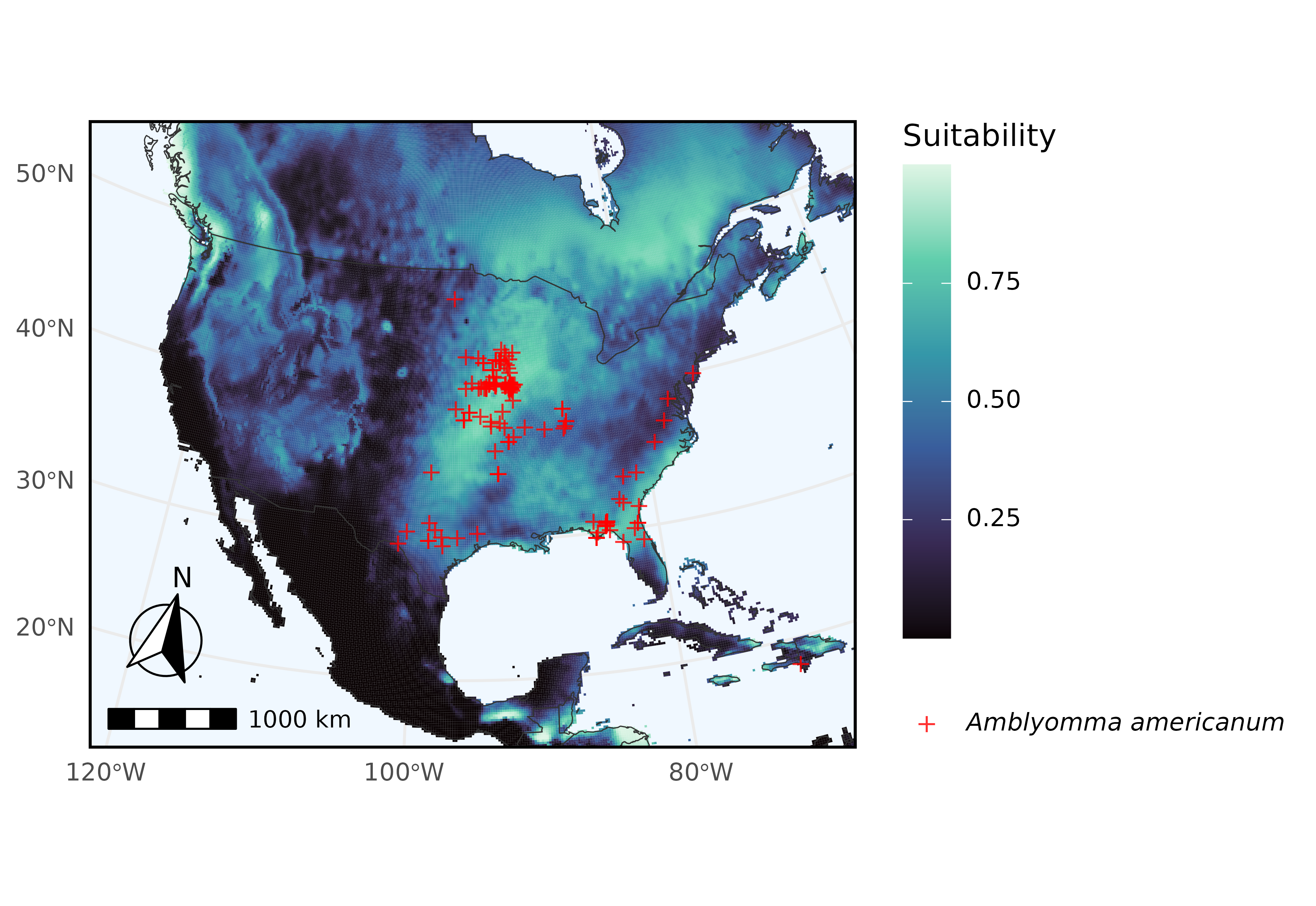
Here we use ggplot2 to plot predicted suitability for Amblyomma americanum, with occurrences overlaid.
pred_df <- as.data.frame(pred$General_consensus[["median"]], xy = TRUE)
occ_points_df <- as.data.frame(occ_geo_points, geom = "XY")
colnames(pred_df) <- c("long", "lat", "suitability")

plot_map <- map_data("world")

tick <- ggplot() +
  geom_tile(
    data = pred_df,
    aes(x = long, y = lat, fill = suitability)
  ) +
  geom_polygon(
    data = plot_map,
    aes(x = long, y = lat, group = group),
    fill = NA, color = "gray20", linewidth = 0.2
  ) +
  geom_point(
    data = occ_points_df,
    aes(x = x, y = y, color = "Amblyomma americanum"),
    shape = "+", size = 3, alpha = 0.8
  ) +
  scale_color_manual(
    name = NULL,
    values = c("Amblyomma americanum" = "red"),
    labels = c("*Amblyomma americanum*")
  ) +
  scale_fill_viridis_c(
    name = "Suitability",
    option = "mako",
    na.value = "aliceblue"
  ) +
  coord_sf(
    crs = "EPSG:5070",
    xlim = c(-130, -60),
    ylim = c(15, 60),
    default_crs = sf::st_crs(4326),
    expand = FALSE
  ) +
  labs(
    x = NULL, y = NULL
  ) +
  annotation_scale(
    location = "bl",
    width_hint = 0.3
  ) +
  annotation_north_arrow(
    location = "bl",
    which_north = "true",
    pad_x = unit(0.1, "in"),
    pad_y = unit(0.3, "in"),
    style = north_arrow_fancy_orienteering
  ) +
  theme_minimal() +
  theme(
    panel.background = element_rect(fill = "aliceblue"),
    panel.border = element_rect(color = "black", fill = NA, linewidth = 1),
    legend.text = element_markdown()
  )

ggsave(
  filename = "figures/tick.png",
  plot = tick,
  width = 6.53,
  height = 4.5,
  dpi = 600,
  create.dir = TRUE
)
#> Warning: Removed 7 rows containing missing values or values outside the scale range
#> (`geom_point()`).