Species search and mapping

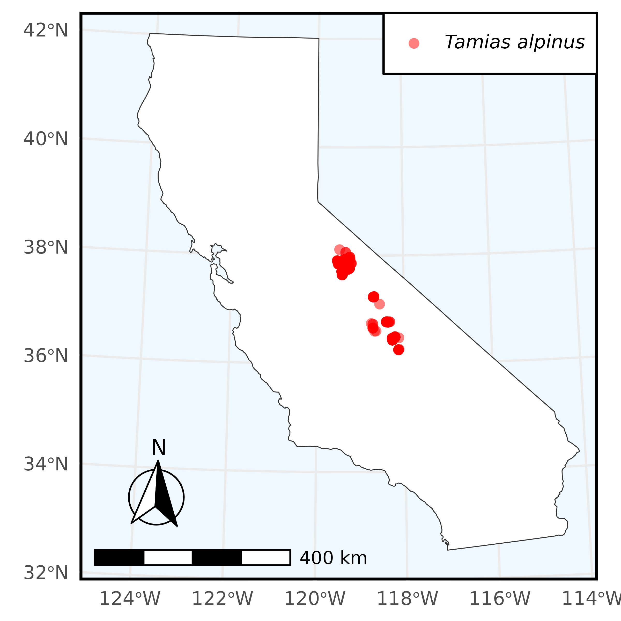
In this example, we perform a simple species search through Arctos and use the data from that query to create a plot with ggplot2. We search for all Tamias alpinus collected in California and stored in the Museum of Vertebrate Zoology’s collection. In our search we request longitude and latitude data, and use that to plot points where specimens were collected over the state of California.

To begin, make sure to load the library:

# install.packages("ArctosR")
# install.packages("ggplot2")
# install.packages("ggspatial")
# install.packages("ggtext")
# install.packages("maps")
# install.packages("sf")

library(ArctosR)
library(ggplot2)
library(ggspatial)
library(ggtext)
library(maps)
library(sf)
#> Linking to GEOS 3.12.1, GDAL 3.8.4, PROJ 9.4.0; sf_use_s2() is TRUE

Exploring Arctos options

First, we can view all parameters we can use to search by on Arctos:

# Request a list of all query parameters.
query_params <- get_query_parameters()

# Explore all parameters.
View(query_params)

The query parameters we are interested in using are: guid_prefix, genus, species, and state_prov.

Next, we can view a list of all parameters we can ask Arctos to return by calling:

# Request a list of all result parameters. These are the names that can show up
# as columns in a dataframe returned by ArctosR.
result_params <- get_result_parameters()

# Explore all parameters.
View(result_params)

The parameters we are interested in returning are: dec_lat and dec_long.

Requesting data

Next we can first ask for a count of how many records we expect our search to return. If this count is not too large we can proceed to request all records. From the response we can get a data.frame using the response_data function.

count <- get_record_count(guid_prefix="MVZ:Mamm", 
                          scientific_name="Tamias alpinus",
                          state_prov="California",
                          api_key=YOUR_API_KEY)

alpinus <- get_records(guid_prefix="MVZ:Mamm", scientific_name="Tamias alpinus",
                       state_prov="California",
                       columns=list("dec_lat", "dec_long"),
                       all_records=TRUE, api_key=YOUR_API_KEY)

alpinus_df <- response_data(alpinus)

# Filter out records which are missing latitude and longitude information
alpinus_df <- alpinus_df[alpinus_df$dec_lat != "" & alpinus_df$dec_long != "", ]

nrow(alpinus_df)
#> [1] 424

Plotting data

Now we use the ggplot2 package to plot the dec_lat and dec_long fields from our data.frame over a map of the state of California.

# Plot of Tamias alpinus sampled in California and currently stored in the
# Museum of Vertebrate Zoology's collection

plot_map <- map_data("state", region=c("California"))

plot <- ggplot(plot_map, aes(long, lat)) +
  geom_polygon(
    aes(group = group), fill = "white", color = "gray20",
    linewidth = .2
  ) +
  geom_jitter(
    data = alpinus_df,
    aes(x = as.numeric(dec_long), y = as.numeric(dec_lat),
    color = "T. alpinus", shape = "T. alpinus"),
    alpha = .5, size = 2.0
  ) +
  scale_color_manual(
    values = c("T. alpinus" = "red"),
    labels = c("*Tamias alpinus*")
  ) +
  scale_shape_manual(
    values = c("T. alpinus" = 16),
    labels = c("*Tamias alpinus*")
  ) +
  labs(
    color = "Species", shape = "Species", x = NULL, y = NULL
  ) +
  coord_sf(
    crs = "+proj=lcc +lat_1=34 +lat_2=40.5 +lat_0=37.25 +lon_0=-119.25 +x_0=0 +y_0=0 +datum=WGS84 +units=m +no_defs",
    xlim = c(-125.5, -113.5),
    ylim = c(32, 42.5),
    default_crs = st_crs(4326),
    expand = FALSE
  ) +
  annotation_scale(
    location = "bl",
    width_hint = 0.4
  ) +
  annotation_north_arrow(
    location = "bl",
    which_north = "true", 
    pad_x = unit(0.2, "in"),
    pad_y = unit(0.3, "in"),
    style = north_arrow_fancy_orienteering
  ) +
  theme_minimal() +
  theme(
    panel.background = element_rect(fill = "aliceblue"),
    panel.border = element_rect(color = "black", fill = NA, linewidth = 1.25),
    legend.position = c(0.998, 0.998),
    legend.justification = c(1, 1),
    legend.background = element_rect(fill = "white"),
    legend.text = element_markdown(),
    legend.title = element_blank()
  )

ggsave(
  filename = "figures/california.png",
  plot = plot,
  width = 4,
  height = 4,
  dpi = 600,
  create.dir = TRUE
)

The result of which is: